Marine aquaculture has the potential to play an important role in the global food supply as a more sustainable protein option than land-based meat production.1Gentry et al. mapped the potential for marine aquaculture globally based on multiple constraints, including ship traffic, dissolved oxygen, bottom depth .2
For this assignment, you are tasked with determining which Exclusive Economic Zones (EEZ) on the West Coast of the US are best suited to developing marine aquaculture for several species of oysters.
Based on previous research, we know that oysters needs the following conditions for optimal growth:
Sea surface temperature: 11-30 °C
Depth: 0-70 meters below sea level
Learning objectives:
Combining vector/raster data
Resampling raster data
Masking raster data
Map algebra
Data
Sea Surface Temperature
We will use average annual sea surface temperature (SST) from the years 2008 to 2012 to characterize the average sea surface temperature within the region. The data we are working with was originally generated from NOAA’s 5km Daily Global Satellite Sea Surface Temperature Anomaly v3.1.
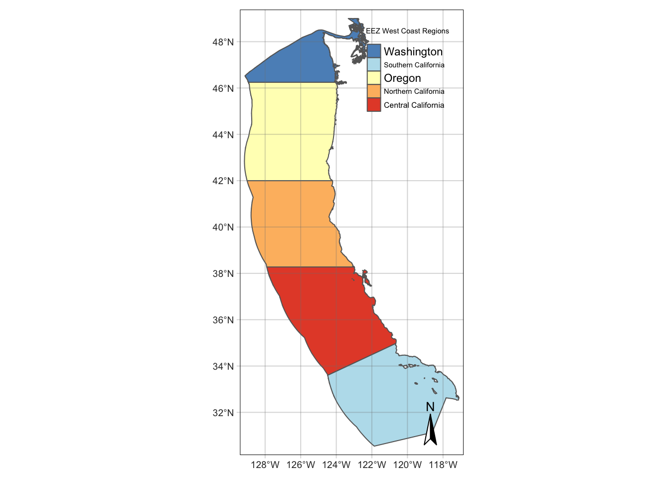
Read in the shape file for the West Coast EEZ (wc_regions_clean.shp)
Read in SST rasters
average_annual_sst_2008.tif
average_annual_sst_2009.tif
average_annual_sst_2010.tif
average_annual_sst_2011.tif
average_annual_sst_2012.tif
Combine SST rasters into a raster stack
Read in bathymetry raster (depth.tif)
Check that data are in the same coordinate reference system
Reproject any data not in the same projection
Code
# Setting my filepathsrootdir <- ("/Users/javipatron/Documents/MEDS/Courses/eds223")data <-file.path(rootdir,"data","assignment4")# Creating the names for each filesst_2008 <-'average_annual_sst_2008.tif'sst_2009 <-"average_annual_sst_2009.tif"sst_2010 <-"average_annual_sst_2010.tif"sst_2011 <-"average_annual_sst_2011.tif"sst_2012 <-"average_annual_sst_2012.tif"depth <-"depth.tif"# Downloading the raster data to a star objectsst_2008 <-rast(file.path(data, sst_2008))sst_2009 <-rast(file.path(data, sst_2009))sst_2010 <-rast(file.path(data, sst_2010))sst_2011 <-rast(file.path(data, sst_2011))sst_2012 <-rast(file.path(data, sst_2012))wc_regions <-st_read(file.path(data, "wc_regions_clean.shp"))
Reading layer `wc_regions_clean' from data source
`/Users/javipatron/Documents/MEDS/Courses/eds223/data/assignment4/wc_regions_clean.shp'
using driver `ESRI Shapefile'
Simple feature collection with 5 features and 5 fields
Geometry type: MULTIPOLYGON
Dimension: XY
Bounding box: xmin: -129.1635 ymin: 30.542 xmax: -117.097 ymax: 49.00031
Geodetic CRS: WGS 84
Code
depth <-rast(file.path(data,depth))# Stack all the rasterall_sst <-c(sst_2008, sst_2009, sst_2010, sst_2011, sst_2012)# Check coordinate reference system#st_crs(wc_regions)#st_crs(depth)#st_crs(all_sst)# Set the new CRSall_sst <-project(all_sst, "EPSG:4326")all_sst
Some legend labels were too wide. These labels have been resized to 0.44, 0.45, 0.49. Increase legend.width (argument of tm_layout) to make the legend wider and therefore the labels larger.
Code
tmap_mode("view")
tmap mode set to interactive viewing
Process Data
Next, we need process the SST and depth data so that they can be combined. In this case the SST and depth data have slightly different resolutions, extents, and positions. We don’t want to change the underlying depth data, so we will need to resample to match the SST data using the nearest neighbor approach.
Find the mean SST from 2008-2012
Convert SST data from Kelvin to Celsius
Crop depth raster to match the extent of the SST raster
note: the resolutions of the SST and depth data do not match
Resample the depth data to match the resolution of the SST data using the nearest neighbor approach.
Check that the depth and SST match in resolution, extent, and coordinate reference system. Can the rasters be stacked?
Code
#Finding the mean mean_sst <- terra::app(all_sst, mean)#Converting to Celsiusmean_sst_c <- (mean_sst -273.15)#Cropping the Depth to just the area of SSTcrop_depth <-crop(depth, mean_sst)class(crop_depth)
[1] "SpatRaster"
attr(,"package")
[1] "terra"
Code
# Re-sample the depth with the needed resolutionnew_depth <- terra::resample(crop_depth, mean_sst_c, method ="near")# Stack both rasters and see if they matchstack_depth_sst <-c(mean_sst_c, new_depth)
Find suitable locations
In order to find suitable locations for marine aquaculture, we’ll need to find locations that are suitable in terms of both SST and depth.
Reclassify SST and depth data into locations that are suitable for Lump sucker fish
hint: set suitable values to 1 and unsuitable values to NA
Find locations that satisfy both SST and depth conditions
hint: create an overlay using the lapp() function multiplying cell values
Code
#Create the matrix for Temperature between 11°C and 30°Ctemp_vector <-c(-Inf, 11, NA, 11, 30, 1,30, Inf, NA)temp_oysters_matrix <-matrix(temp_vector, ncol=3, byrow = T)# Reclassify the SST raster of °Ctemp_oysters <-classify(mean_sst_c, temp_oysters_matrix)#Create the matrix for Depth between 0 & -70depth_vector <-c(-Inf, -70, NA, -70, 0, 1,0, Inf, NA)depth_oysters_matrix <-matrix(depth_vector, ncol=3, byrow = T)# Reclassify the SST raster of depthdepth_oysters <-classify(new_depth, depth_oysters_matrix, include.lowest = T)# Combine the two rastermatrixes <-c(depth_oysters, temp_oysters)# Rename the matrixes attributesnames(matrixes) <-c("temp_matx","depth_matx")#Combine both matrixescombined_matrix_stack <-c(matrixes, stack_depth_sst)
Code
#Find the locations where the oysters have a 1 in the pixel.check_condition <-function(x,y){return(x * y) }temp_conditions <-lapp(combined_matrix_stack[[c(1,3)]], fun = check_condition)depth_conditions <-lapp(combined_matrix_stack[[c(2,4)]], fun = check_condition)tm_shape(temp_conditions) +tm_raster(title ="Sea Temp °C") +tm_graticules(alpha =0.3) +tm_compass(position =c("right", "top")) +tm_layout(legend.outside =TRUE,frame = T)
Variable(s) "NA" contains positive and negative values, so midpoint is set to 0. Set midpoint = NA to show the full spectrum of the color palette.
Now lets create the mask of both conditions
Code
suitable_conditions <-lapp(matrixes[[c(1,2)]], fun = check_condition)print(suitable_conditions)
class : SpatRaster
dimensions : 480, 408, 1 (nrow, ncol, nlyr)
resolution : 0.04165905, 0.04165905 (x, y)
extent : -131.9848, -114.9879, 29.99208, 49.98842 (xmin, xmax, ymin, ymax)
coord. ref. : lon/lat WGS 84 (EPSG:4326)
source(s) : memory
name : lyr1
min value : 1
max value : 1
Determine the most suitable EEZ
We want to determine the total suitable area within each EEZ in order to rank zones by priority. To do so, we need to find the total area of suitable locations within each EEZ.
Select suitable cells within West Coast EEZs
Find area of grid cells
Find the total suitable area within each EEZ
hint: it might be helpful to rasterize the EEZ data
Find the percentage of each zone that is suitable
hint it might be helpful to join the suitable area by region onto the EEZ vector data
Code
cell_ezz <-cellSize(suitable_conditions, unit ='km', transform =TRUE)rast_ezz <-rasterize(wc_regions, suitable_conditions, field='rgn')mask_ezz <-mask(rast_ezz, suitable_conditions)suitable_area <-zonal(cell_ezz, mask_ezz, sum )joined_area <-left_join(wc_regions, suitable_area, by ='rgn') |>mutate(area_suitkm2 = area,percentage = (area_suitkm2 / area_km2) *100,.before = geometry)
Visualize results
Now that we have results, we need to present them!
Create the following maps:
Total suitable area by region
Percent suitable area by region
Code
tm_shape(joined_area) +tm_polygons(col ="area", palette ="RdYlBu", legend.reverse = T, title ="Area (km2)") +tm_shape(wc_regions) +tm_polygons(alpha =0.5) +tm_layout(legend.outside =TRUE,main.title.size =1,main.title =paste("Total Suitable area per EEZ for: Oysters"),frame = T)
As you can see in the maps above the most suitable areas for the oysters are the northerner regions with a 3 to 3.5 % of the entire EEZ region. As the assignments states the sea surface temperature that the oysters like are between the 11-30 °C, and for the depth is between 0-70 meters below sea level, which are pretty specific. Thus, this results can give us hints on how the Economic Exclusive Zones help those species, and we can compare to other EEZ or other species of the US West Coast.
Broaden your workflow!
Now that you’ve worked through the solution for one group of species, let’s update your workflow to work for other species. Please create a function that would allow you to reproduce your results for other species. Your function should be able to do the following:
Accept temperature and depth ranges and species name as inputs
Create maps of total suitable area and percent suitable area per EEZ with the species name in the title
Run your function for a species of your choice! You can find information on species depth and temperature requirements on SeaLifeBase. Remember, we are thinking about the potential for marine aquaculture, so these species should have some reasonable potential for commercial consumption.
1. The species name has to be in quotes. The Default value is “NAME”.
2. The depth has to include the negative sign for the maximum depth.
Default; Min: 0, Max: -5468.
3. The Temperature is in °C .
Default; Min: 5, Max: 30).
Code
find_my_happy_place()
Simple feature collection with 5 features and 5 fields
Geometry type: MULTIPOLYGON
Dimension: XY
Bounding box: xmin: -129.1635 ymin: 30.542 xmax: -117.097 ymax: 49.00031
Geodetic CRS: WGS 84
rgn rgn_key area_km2 happy_area_km2 happy_(%)
1 Southern California CA-S 206860.78 205730.95 99.45382
2 Central California CA-C 202738.33 201478.95 99.37882
3 Oregon OR 179994.06 178650.46 99.25353
4 Northern California CA-N 164378.81 162975.61 99.14636
5 Washington WA 66898.31 64695.95 96.70790
geometry
1 MULTIPOLYGON (((-120.6505 3...
2 MULTIPOLYGON (((-122.9928 3...
3 MULTIPOLYGON (((-123.4318 4...
4 MULTIPOLYGON (((-124.2102 4...
5 MULTIPOLYGON (((-122.7675 4...
[1] "*Conclusion:* For the species NAME the most suitable region is Southern California with 205730.95 km2 of 'happy' area."
Code
# Try your species!! find_my_happy_place("Turtle", 13, 28, 0, -290)
Simple feature collection with 5 features and 5 fields
Geometry type: MULTIPOLYGON
Dimension: XY
Bounding box: xmin: -129.1635 ymin: 30.542 xmax: -117.097 ymax: 49.00031
Geodetic CRS: WGS 84
rgn rgn_key area_km2 happy_area_km2 happy_(%)
1 Southern California CA-S 206860.78 10890.3024 5.26455645
2 Central California CA-C 202738.33 360.9648 0.17804468
3 Washington WA 66898.31 29.1610 0.04359004
4 Oregon OR 179994.06 NA NA
5 Northern California CA-N 164378.81 NA NA
geometry
1 MULTIPOLYGON (((-120.6505 3...
2 MULTIPOLYGON (((-122.9928 3...
3 MULTIPOLYGON (((-122.7675 4...
4 MULTIPOLYGON (((-123.4318 4...
5 MULTIPOLYGON (((-124.2102 4...
[1] "*Conclusion:* For the species Turtle the most suitable region is Southern California with 10890.3 km2 of 'happy' area."
Footnotes
Hall, S. J., Delaporte, A., Phillips, M. J., Beveridge, M. & O’Keefe, M. Blue Frontiers: Managing the Environmental Costs of Aquaculture (The WorldFish Center, Penang, Malaysia, 2011).↩︎
Gentry, R. R., Froehlich, H. E., Grimm, D., Kareiva, P., Parke, M., Rust, M., Gaines, S. D., & Halpern, B. S. Mapping the global potential for marine aquaculture. Nature Ecology & Evolution, 1, 1317-1324 (2017).↩︎
GEBCO Compilation Group (2022) GEBCO_2022 Grid (doi:10.5285/e0f0bb80-ab44-2739-e053-6c86abc0289c).↩︎
Citation
BibTeX citation:
@online{patrón2022,
author = {Patrón, Javier},
title = {Marine {Aquaculture}},
date = {2022-12-16},
url = {https://github.com/javipatron},
langid = {en}
}