“In February 2021, the state of Texas suffered a major power crisis, which came about as a result of three severe winter storms sweeping across the United States on February 10–11, 13–17, and 15–20.”1 For more background, check out these engineering and political perspectives.
The tasks in this post are: - Estimating the number of homes in Houston that lost power as a result of the first two storms
- Investigating if socioeconomic factors are predictors of communities recovery from a power outage
The analysis will be based on remotely-sensed night lights data, acquired from the Visible Infrared Imaging Radiometer Suite (VIIRS) onboard the Suomi satellite. In particular, you will use the VNP46A1 to detect differences in night lights before and after the storm to identify areas that lost electric power.
To determine the number of homes that lost power, you link (spatially join) these areas with OpenStreetMap data on buildings and roads.
To investigate potential socioeconomic factors that influenced recovery, you will link your analysis with data from the US Census Bureau.
Spatial Skills:
Load vector/raster data
Simple raster operations
Simple vector operations
Spatial joins
Data
Night lights
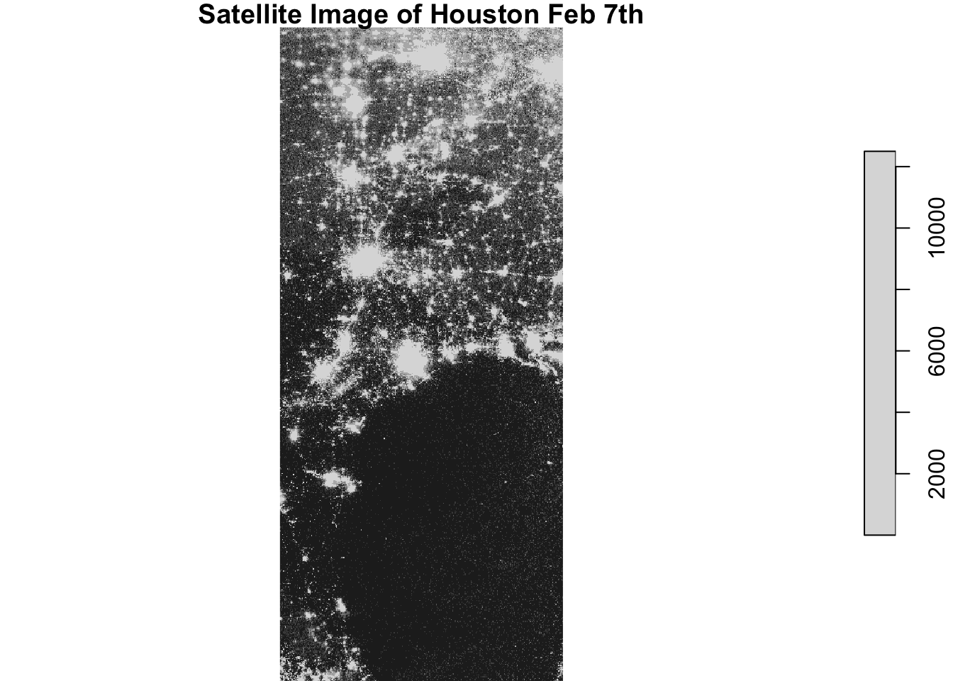
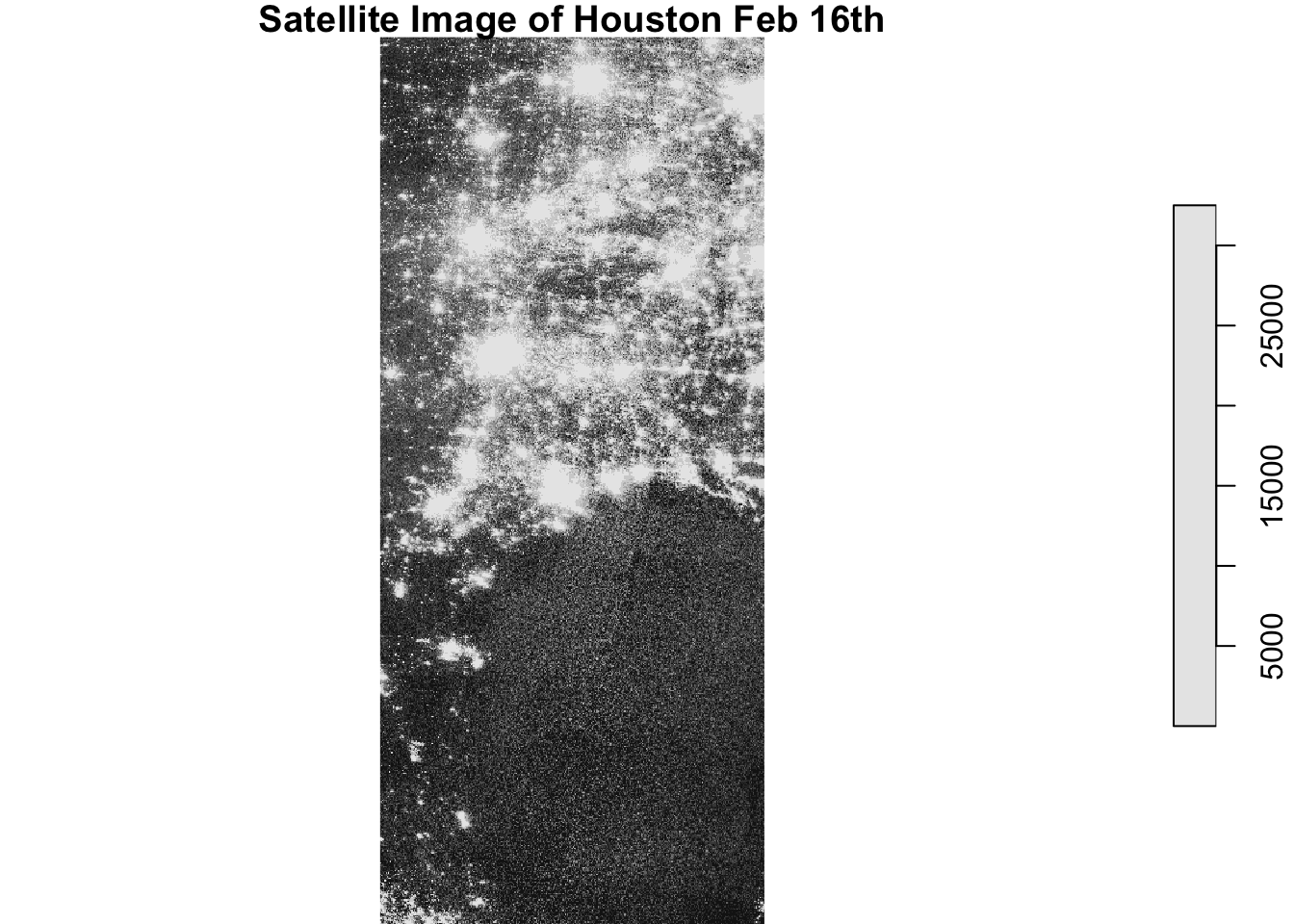
Use NASA’s Worldview to explore the data around the day of the storm. There are several days with too much cloud cover to be useful, but 2021-02-07 and 2021-02-16 provide two clear, contrasting images to visualize the extent of the power outage in Texas.
VIIRS data is distributed through NASA’s Level-1 and Atmospheric Archive & Distribution System Distributed Active Archive Center (LAADS DAAC). Many NASA Earth data products are distributed in 10x10 degree tiles in sinusoidal equal-area projection. Tiles are identified by their horizontal and vertical position in the grid. Houston lies on the border of tiles h08v05 and h08v06. We therefore need to download two tiles per date.
Roads
Typically highways account for a large portion of the night lights observable from space (see Google’s Earth at Night). To minimize falsely identifying areas with reduced traffic as areas without power, we will ignore areas near highways.
OpenStreetMap (OSM) is a collaborative project which creates publicly available geographic data of the world. Ingesting this data into a database where it can be subsetted and processed is a large undertaking. Fortunately, third party companies redistribute OSM data. We used Geofabrik’s download sites to retrieve a shape file of all highways in Texas and prepared a Geopackage (.gpkg file) containing just the subset of roads that intersect the Houston metropolitan area.
gis_osm_roads_free_1.gpkg
Houses
We can also obtain building data from OpenStreetMap. We again downloaded from Geofabrick and prepared a GeoPackage containing only houses in the Houston metropolitan area.
gis_osm_buildings_a_free_1.gpkg
Socioeconomic
We cannot readily get socioeconomic information for every home, so instead we obtained data from the U.S. Census Bureau’s American Community Survey for census tracts in 2019. The folderACS_2019_5YR_TRACT_48.gdb is an ArcGIS “file geodatabase”, a multi-file proprietary format that’s roughly analogous to a GeoPackage file.
The geodatabase contains a layer holding the geometry information, separate from the layers holding the ACS attributes. You have to combine the geometry with the attributes to get a feature layer that sf can use.
Assignment
Find locations of blackouts
For improved computational efficiency and easier interoperability with sf, we will use the stars package for raster handling.
Code
# Setting my filepathsrootdir <- ("/Users/javipatron/Documents/MEDS/Courses/eds223")datatif <-file.path(rootdir,"data","VNP46A1")data <-file.path(rootdir,"data")#Creating the names for each filenightlight1 <-'VNP46A1.A2021038.h08v05.001.2021039064328.tif'nightlight2 <-'VNP46A1.A2021038.h08v06.001.2021039064329.tif'nightlight3 <-'VNP46A1.A2021047.h08v05.001.2021048091106.tif'nightlight4 <-'VNP46A1.A2021047.h08v06.001.2021048091105.tif'#Downloading the raster data to a star objectone <-read_stars(file.path(datatif, nightlight1))two <-read_stars(file.path(datatif, nightlight2))three <-read_stars(file.path(datatif,nightlight3))four <-read_stars(file.path(datatif,nightlight4))
Code
#Combine tiles to have the full sizelights_off <-st_mosaic(one,two)lights_on <-st_mosaic(three,four)plot(lights_off, main="Satellite Image of Houston Feb 7th")
downsample set to 6
Code
plot(lights_on, main="Satellite Image of Houston Feb 16th")
downsample set to 6
Create a blackout mask
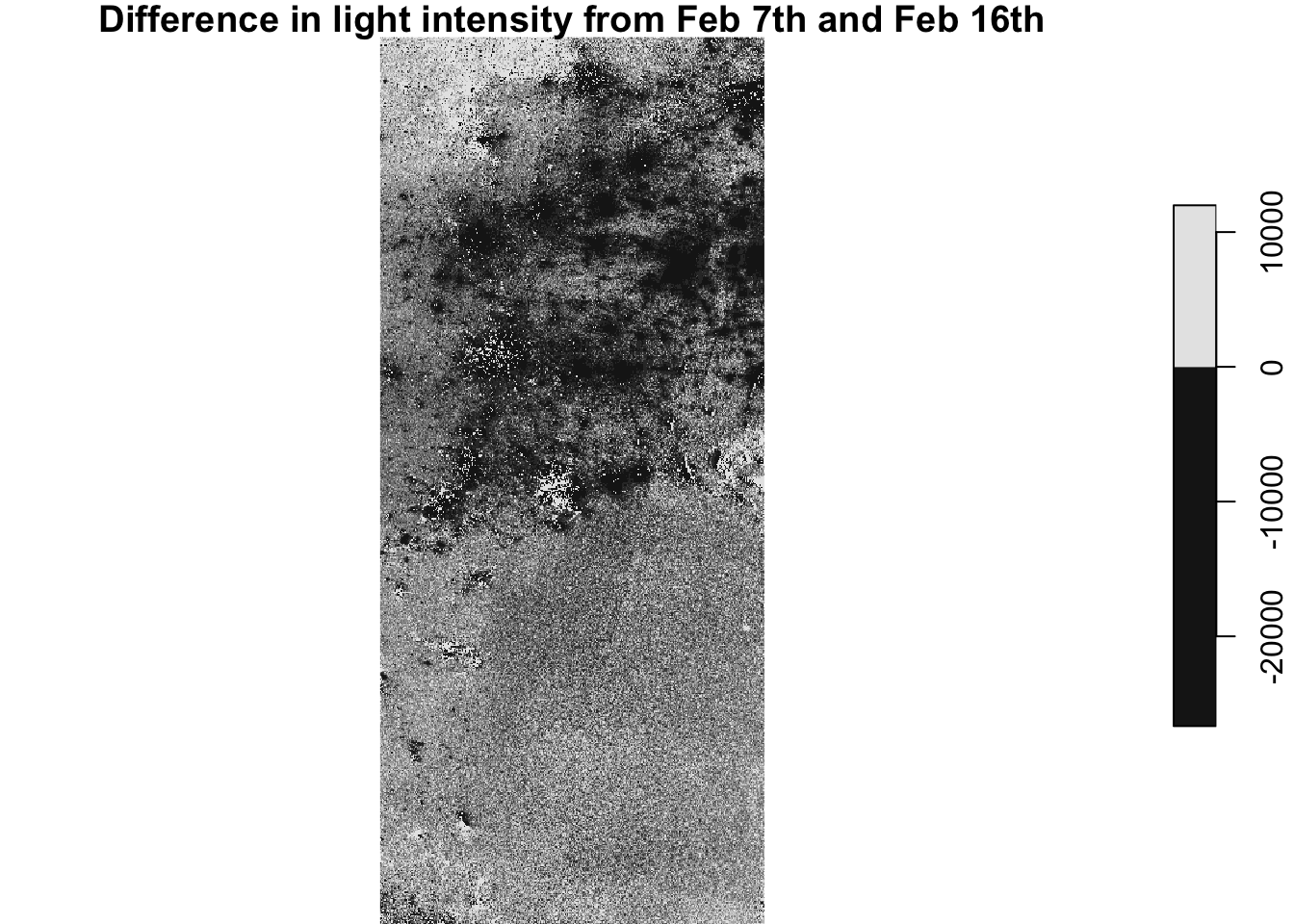
Find the change in night lights intensity (presumably) caused by the storm Response: The change on the mean from the second date (All lights) goes from 13.86 down 12.13939, on the first date (Outrage)
Reclassify the difference raster, assuming that any location that experienced a drop of more than 200 nW cm-2sr-1 experienced a blackout
Assign NA to all locations that experienced a drop of less than 200 nW cm-2sr-1
Code
#Create a new raster that has the difference of the values from the Feb 7th (Lights Off) raster, and the 16th (Lights On) raster. This will just have the difference of the attribute value on each pixelraster_diff <- lights_off - lights_onplot(raster_diff, main="Difference in light intensity from Feb 7th and Feb 16th")
downsample set to 6
Vectorize the mask
Using st_as_sf() to vectorize the blackout mask
Fixing any invalid geometries by using st_make_valid
Code
# Converts the non-spatial star object (.tif) file to an sf object. An sf object will have an organizing structure that will have the geom column and the layer as attribuesblackout <-st_as_sf(raster_diff)summary(blackout)
VNP46A1.A2021038.h08v05.001.2021039064328.tif geometry
Min. : 200.0 POLYGON :24950
1st Qu.: 262.0 epsg:4326 : 0
Median : 359.0 +proj=long...: 0
Mean : 543.8
3rd Qu.: 563.0
Max. :65512.0
Crop the vectorized map to our region of interest.
Define the Houston metropolitan area with the following coordinates
Turn these coordinates into a polygon using st_polygon
Convert the polygon into a simple feature collection using st_sfc() and assign a CRS
hint: because we are using this polygon to crop the night lights data it needs the same CRS
Crop (spatially subset) the blackout mask to our region of interest
Re-project the cropped blackout dataset to EPSG:3083 (NAD83 / Texas Centric Albers Equal Area)
Code
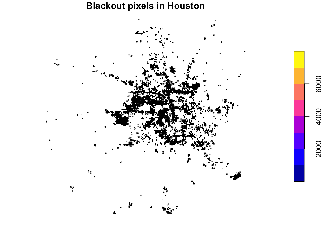
#Create vectors for the desired CRSlon =c(-96.5, -96.5, -94.5, -94.5,-96.5)lat =c(29, 30.5, 30.5, 29, 29)#Create an array or matrix with those vectors coordinates_array <-cbind(lon,lat)#Creating a polygon with the st_polygon function but the coordinates_array has to be in the form of a list so the st_polygon can read it.houston_polygon <-st_polygon(list(coordinates_array))# Create a simple feature geometry list column, and add coordinate reference system so you can "speak" the same language than your recent blackout objecthouston_geom <-st_sfc(st_polygon(list(coordinates_array)), crs =4326)# Indexing or Cropping the blackout sf object with just the houston geometery polygon. houston_blackout_subset <- blackout[houston_geom,]# Re-project the cropped blackout dataset with a new CRS (EPSG:3083) (NAD83 / Texas Centric Albers Equal Area)houston_projection <-st_transform(houston_blackout_subset,"EPSG:3083")
Code
plot(houston_blackout_subset, main ="Blackout pixels in Houston")
Exclude highways from blackout mask
The roads geopackage includes data on roads other than highways. However, we can avoid reading in data we don’t need by taking advantage of st_read’s ability to subset using a SQL query.
Define SQL query
Load just highway data from geopackage using st_read
Reproject data to EPSG:3083
Identify areas within 200m of all highways using st_buffer
Find areas that experienced blackouts that are further than 200m from a highway
Code
#Reading the data with format .gpkgquery <-"SELECT * FROM gis_osm_roads_free_1 WHERE fclass='motorway'"highways <-st_read(file.path(data, "gis_osm_roads_free_1.gpkg"), query = query)
Reading query `SELECT * FROM gis_osm_roads_free_1 WHERE fclass='motorway''
from data source `/Users/javipatron/Documents/MEDS/Courses/eds223/data/gis_osm_roads_free_1.gpkg'
using driver `GPKG'
Simple feature collection with 6085 features and 10 fields
Geometry type: LINESTRING
Dimension: XY
Bounding box: xmin: -96.50429 ymin: 29.00174 xmax: -94.39619 ymax: 30.50886
Geodetic CRS: WGS 84
Code
#Transform that new sf object with the CRS we have been using, so we stay in the same space.highways_3083 <-st_transform(highways, "EPSG:3083")
Code
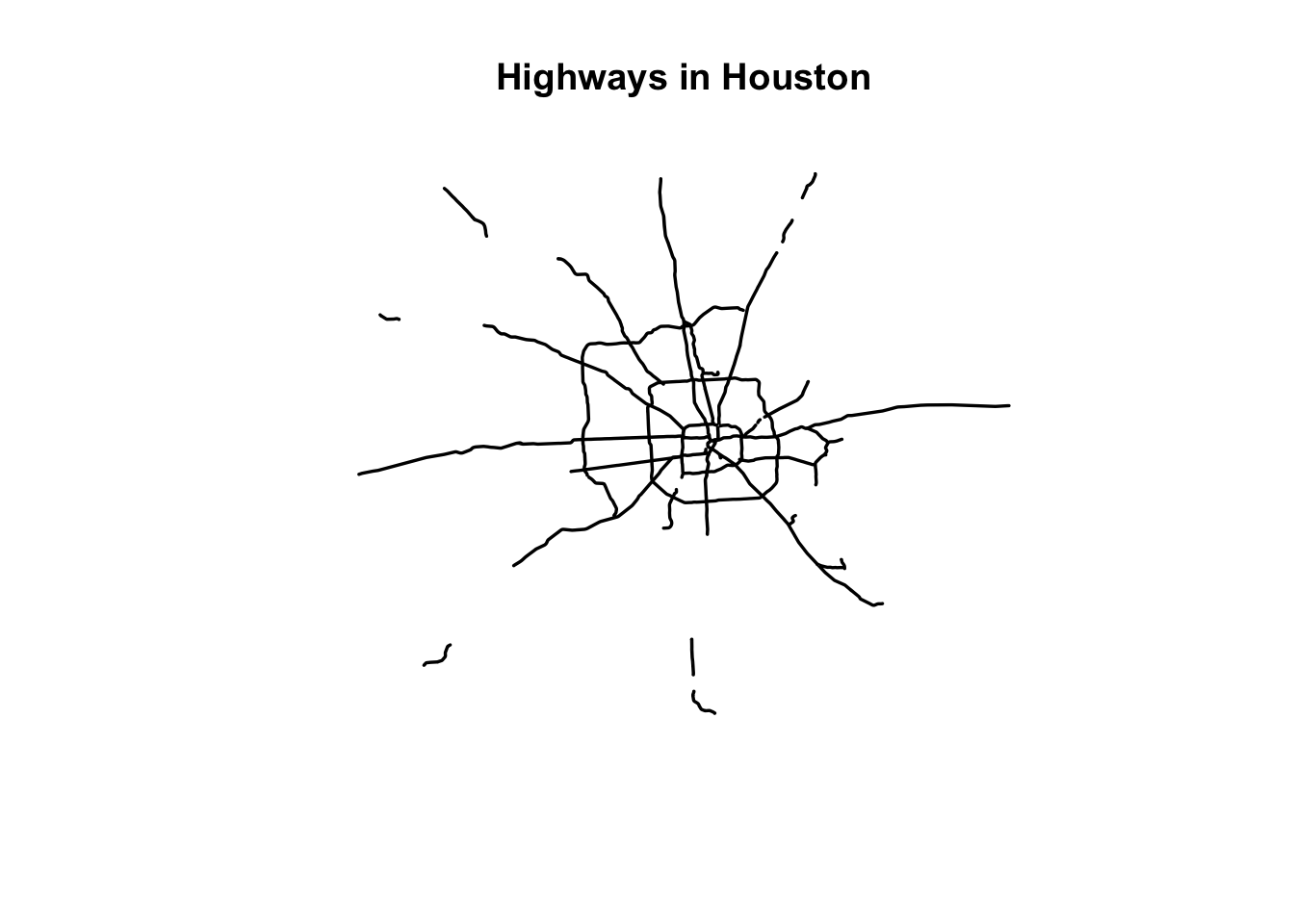
#Create a buffer that contains all the roads, including the 200 meters across the roads.# BUT, to make a buffer object we need to first create a union of all those rows (highways), so we can use the st_buffer function...highways_union <-st_union(highways_3083)highways_buffer <-st_buffer(x = highways_union,dist =200)plot(highways_buffer, main ="Highways in Houston")
Code
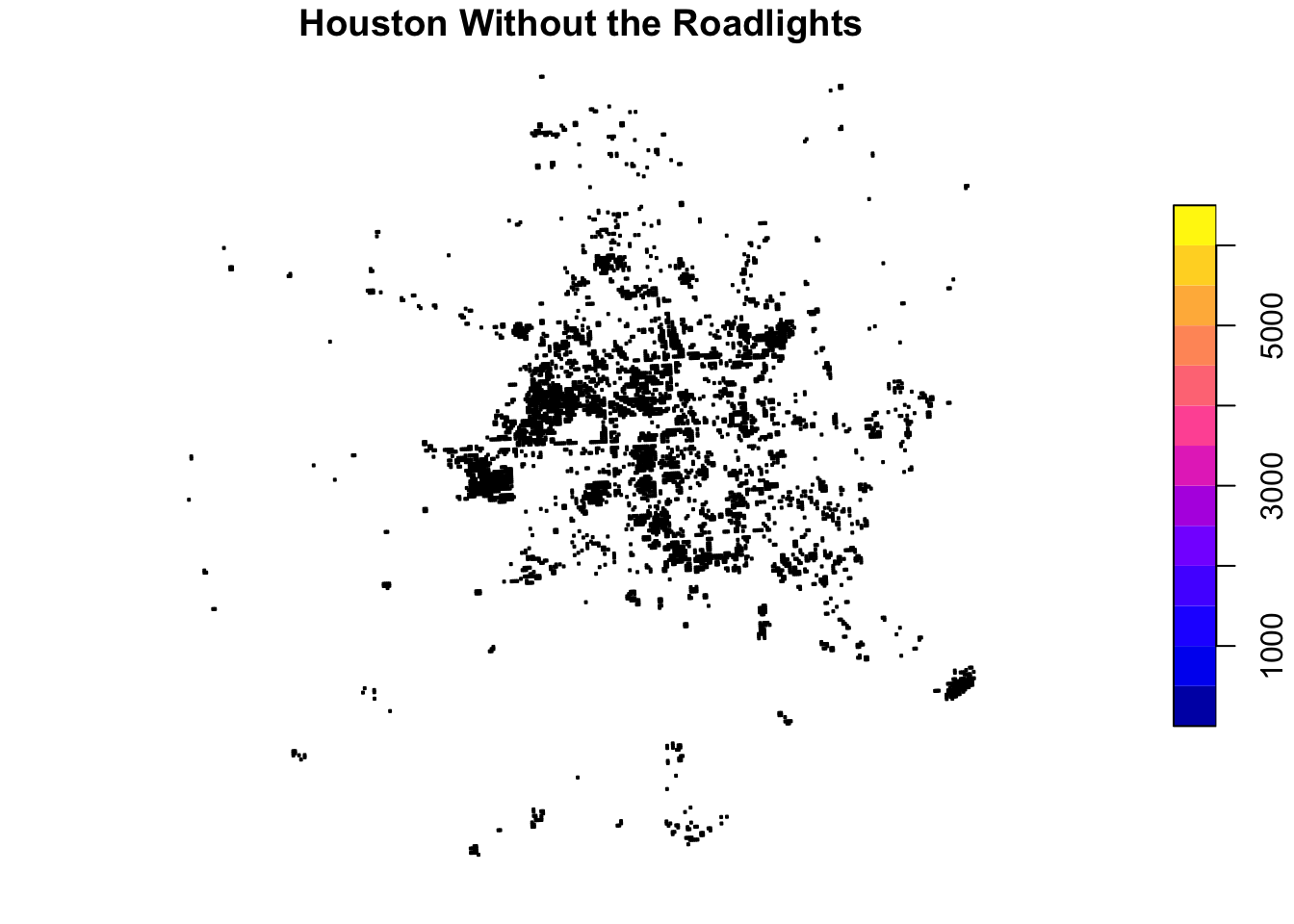
# Use the buffer to subtract those entire pixels or "rows" from the houston projection sf object.houston_out <- houston_projection[highways_buffer, op = st_disjoint]plot(houston_out,main="Houston Without the Roadlights")
Find homes impacted by blackouts
Load buildings dataset using st_read and the following SQL query to select only residential buildings
hint: reproject data to EPSG:3083
Code
#Read the dataquery2 <-"SELECT * FROM gis_osm_buildings_a_free_1 WHERE (type IS NULL AND name IS NULL) OR type in ('residential', 'apartments', 'house', 'static_caravan', 'detached')"buildings <-st_read(file.path(data, "gis_osm_buildings_a_free_1.gpkg"), query = query2)
Reading query `SELECT * FROM gis_osm_buildings_a_free_1 WHERE (type IS NULL AND name IS NULL) OR type in ('residential', 'apartments', 'house', 'static_caravan', 'detached')'
from data source `/Users/javipatron/Documents/MEDS/Courses/eds223/data/gis_osm_buildings_a_free_1.gpkg'
using driver `GPKG'
Simple feature collection with 475941 features and 5 fields
Geometry type: MULTIPOLYGON
Dimension: XY
Bounding box: xmin: -96.50055 ymin: 29.00344 xmax: -94.53285 ymax: 30.50393
Geodetic CRS: WGS 84
Find homes in blackout areas
Filter to homes within blackout areas.
Tip: You can use [ ] option to subtract those geometries from the building sf object that do not correspond to the Houston area. Or you can use the st_filter.
Count number of impacted homes.
Tip: The total number of impacted houses when using st_filter or [ ] is 139,148. This could vary depending on how the st_filter considers the limits and borders of the geometries. The default method when using st_filter is st_intersects.
Code
#Count number of housesdim(homes_blackout_join)[1]
[1] 139148
Investigate socioeconomic factors
Load ACS data
Use st_read() to load the geodatabase layers
Geometries are stored in the ACS_2019_5YR_TRACT_48_TEXAS layer
Income data is stored in the X19_INCOME layer
Select the median income field B19013e1
hint: reproject data to EPSG:3083
Code
#Read the data and understand the data layersst_layers(file.path(data, "ACS_2019_5YR_TRACT_48_TEXAS.gdb"))
Driver: OpenFileGDB
Available layers:
layer_name geometry_type features fields crs_name
1 X01_AGE_AND_SEX NA 5265 719 <NA>
2 X02_RACE NA 5265 433 <NA>
3 X03_HISPANIC_OR_LATINO_ORIGIN NA 5265 111 <NA>
4 X04_ANCESTRY NA 5265 665 <NA>
5 X05_FOREIGN_BORN_CITIZENSHIP NA 5265 1765 <NA>
6 X06_PLACE_OF_BIRTH NA 5265 1221 <NA>
7 X07_MIGRATION NA 5265 1793 <NA>
8 X08_COMMUTING NA 5265 2541 <NA>
9 X09_CHILDREN_HOUSEHOLD_RELATIONSHIP NA 5265 263 <NA>
10 X10_GRANDPARENTS_GRANDCHILDREN NA 5265 373 <NA>
11 X11_HOUSEHOLD_FAMILY_SUBFAMILIES NA 5265 781 <NA>
12 X12_MARITAL_STATUS_AND_HISTORY NA 5265 759 <NA>
13 X13_FERTILITY NA 5265 399 <NA>
14 X14_SCHOOL_ENROLLMENT NA 5265 779 <NA>
15 X15_EDUCATIONAL_ATTAINMENT NA 5265 715 <NA>
16 X16_LANGUAGE_SPOKEN_AT_HOME NA 5265 871 <NA>
17 X17_POVERTY NA 5265 3941 <NA>
18 X18_DISABILITY NA 5265 893 <NA>
19 X19_INCOME NA 5265 3045 <NA>
20 X20_EARNINGS NA 5265 2185 <NA>
21 X21_VETERAN_STATUS NA 5265 565 <NA>
22 X22_FOOD_STAMPS NA 5265 243 <NA>
23 X23_EMPLOYMENT_STATUS NA 5265 1625 <NA>
24 X25_HOUSING_CHARACTERISTICS NA 5265 4415 <NA>
25 X27_HEALTH_INSURANCE NA 5265 1593 <NA>
26 X28_COMPUTER_AND_INTERNET_USE NA 5265 385 <NA>
27 X29_VOTING_AGE_POPULATION NA 5265 35 <NA>
28 X99_IMPUTATION NA 5265 783 <NA>
29 X24_INDUSTRY_OCCUPATION NA 5265 2107 <NA>
30 X26_GROUP_QUARTERS NA 5265 3 <NA>
31 TRACT_METADATA_2019 NA 35976 2 <NA>
32 ACS_2019_5YR_TRACT_48_TEXAS Multi Polygon 5265 15 NAD83
Determine which census tracts experienced blackouts.
Join the income data to the census tract geometries
hint: make sure to join by geometry ID
Spatially join census tract data with buildings determined to be impacted by blackouts
Find which census tracts had blackouts
Code
#Create a big sf that has the income information and its geometryincome_geom <-left_join(texas_geom, texas_income, by ="GEOID_Data")#Create an new sf that adds the income information to just the blackout sf object that we previously had. In this step I learned that if you use st_join will give you a different number and result than st_filter or [ ]#blackout_income_join <- st_join(homes_blackout_join, income_geom)blackout_join <- income_geom[homes_blackout_join,]#Print those Census Tracts a had blackouts. Im printing the number and the namelength(unique(blackout_join$NAMELSAD))
[1] 711
Code
#unique(blackout_join$NAMELSAD)
Compare incomes of impacted tracts to unimpacted tracts.
Create a map of median income by census tract, designating which tracts had blackouts
Plot the distribution of income in impacted and unimpacted tracts
Write approx. 100 words summarizing your results and discussing any limitations to this study
Code
#Creating a list of tracts and counties that were affected by the blackoutblackout_tracts <-unique(blackout_join$TRACTCE)blackout_counties <-unique(blackout_join$COUNTYFP)#Creating a Data Frames that includes only the rows that have the county affected by using the geom from blackout_tracts. One with the Counties and the other one with the Tracts.tracts_affected <- income_geom |>filter(TRACTCE %in% blackout_tracts)counties_affected <- income_geom |>filter(COUNTYFP %in% blackout_counties)#Create a map were the base is the counties of Houston, then fill the color with the income_median column we created with "B19013e1", and then highlight the counties that were had building affected from our datasetmap <-tm_shape(counties_affected) +tm_fill(col ="income_median", palette ="BrBG") +tm_borders() +tm_shape(blackout_join) +tm_fill(col ="pink", alpha=0.3) +tm_layout(legend.outside = T,main.title ="Median Income by Census Tract",frame = T,title ="*Affected areas in pink*") +tm_compass(type ="arrow", position =c("left", "top")) +tm_scale_bar()tmap_mode("view")